Linear Regression Demystified: A Gentle Introduction with Python Examples

Introduction

I have my share of struggles when it comes to understanding models. The equations, the terminology, the fear of getting lost in layers of abstract math. But I’ve also learned that the more you untangle the concepts yourself, the more serotonin it brings. There’s a strange comfort in finally understanding what once felt like gibberish.

When I first heard the term “Linear Regression” it felt mathematical and distant. But the idea behind it is surprisingly human. Imagine you’re trying to predict your friend’s happiness based on how much chocolate they eat. More chocolate, more smiles? That’s a linear relationship. And that’s the core of Linear Regression, understanding how one thing affects another.

So, this blog is not from an expert, but from just a beginner who is learning alongside you.

---

What is Linear Regression?

In a sentence, Linear Regression is a supervised learning algorithm used for predicting a continuous outcome based on one or more input variables.

It answers a simple question:

How does a change in X affect Y?

It assumes there’s a straight-line relationship between your inputs and outputs. That assumption might seem limiting, but it’s powerful enough to model many real-world problems.

Imagine you want to guess how many candies you’ll get if you do some chores.

• If you do more chores, you get more candies.
• If you do fewer chores, you get fewer candies.

Linear regression is like drawing a straight line that helps you guess exactly how many candies you’ll get based on how many chores you do.

Sometimes, you look at just one thing (like chores) to guess candies. That’s simple linear regression. Other times, you look at many things (like chores, being nice, and sharing toys) to guess candies. That’s multiple linear regression.

So basically, it helps you guess one thing by looking at one or more things, assuming the relationship is like a straight line. If you can draw a straight line through your points, it’s a good way to guess.

Some common examples:

• Predicting the price of a house based on its size
• Estimating a student’s final grade based on study hours
• Forecasting rainfall based on humidity levels

If the relationship looks like a line when plotted, Linear Regression is usually a good start.

---

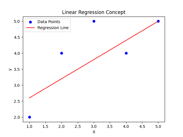
The Linear Equation

At its heart, Linear Regression tries to fit data to this equation:

y = β₀ + β₁x

Where:

• y = predicted outcome (dependent variable)
• x = input feature (independent variable)
• β₁ = slope (how much y changes per unit x)
• β₀ = intercept (value of y when x is 0)

This is the line that tries to pass through the cloud of your data in a way that best represents it.

---

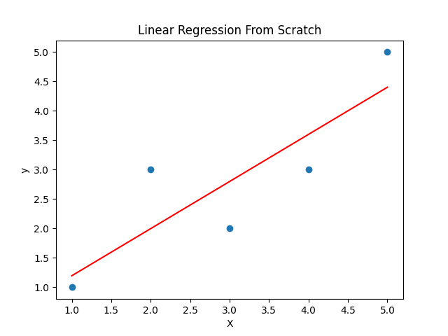
From-Scratch Python Implementation

import numpy as np
import matplotlib.pyplot as plt


# Simple dataset
X = np.array([1, 2, 3, 4, 5])
y = np.array([1, 3, 2, 3, 5])


# Initial guesses
m = 0
b = 0
L = 0.01  # Learning rate
epochs = 1000
n = float(len(X))


# Gradient Descent Loop
for i in range(epochs):
    y_pred = m * X + b
    D_m = (-2/n) * sum(X * (y - y_pred))
    D_b = (-2/n) * sum(y - y_pred)
    m = m - L * D_m
    b = b - L * D_b


print(f"Slope: {m}, Intercept: {b}")


# Plotting
plt.scatter(X, y)
plt.plot(X, m*X + b, color='red')
plt.title("Linear Regression From Scratch")
plt.xlabel("X")
plt.ylabel("y")
plt.show()

---

Using Scikit-Learn

Scikit-learn gives us a cleaner way to do the same:

from sklearn.linear_model import LinearRegression
import numpy as np
import matplotlib.pyplot as plt


X = np.array([[1], [2], [3], [4], [5]])
y = np.array([1, 3, 2, 3, 5])


model = LinearRegression()
model.fit(X, y)


print(f"Intercept: {model.intercept_}")
print(f"Slope: {model.coef_}")


y_pred = model.predict(X)


plt.scatter(X, y)
plt.plot(X, y_pred, color='red')
plt.title("Linear Regression using scikit-learn")
plt.show()

---

---

Now, no model produces perfect results every time. But we can measure its performance and improve it using a few key steps. Let’s dive into how that works.

Minimizing Errors and Optimization:

The Cost Function

How do we know if a line fits well?

We measure the error: the difference between what the model predicts and what the actual values are. A common way to do this is the Mean Squared Error (MSE):

MSE = (1/n) * Σ(yᵢ - ŷᵢ)²

• yᵢ: actual value
• ŷᵢ: predicted value
• n: total number of observations

The smaller the MSE, the better the line fits.

---

Understanding Prediction Error (aka Loss)

Imagine you’re trying to guess your friend’s age, and she is 10 years old.

If you guess 8, your error is 2 years. If you guess 12, you’re also 2 years off. That difference between what you guessed and what’s true is called the error.

In Linear Regression, we do the same thing. For every prediction, we compare it with the real answer. But instead of just error, we use something called Mean Squared Error (MSE) to see how well (or badly) our guesses are doing.

How is the Loss (Error) Calculated?

Let’s say you tried to guess someone’s weight based on their height. You had 3 people:

Height (X)	Actual Weight (y)	Predicted Weight (ŷ)
1.5m	50kg	52kg
1.6m	55kg	54kg
1.8m	65kg	63kg

To calculate MSE:

1. Find the difference between actual and predicted:

   • (50 - 52) = -2
   • (55 - 54) = 1
   • (65 - 63) = 2

2. Square each error:

   • (-2)² = 4
   • 1² = 1
   • 2² = 4

3. Add them up: 4 + 1 + 4 = 9

4. Divide by number of observations (3): MSE = 9 / 3 = 3

That’s our loss. Smaller MSE = better guesses.

Forward Pass and Backward Pass

Imagine your model is a little robot that guesses outcomes.

Forward Pass This is when the robot makes a guess. It takes the input x and does the math:

y = m*x + b

Example: If m = 2, b = 3, and x = 4, then: y = 2*4 + 3 = 11

Backward Pass (Learning Time!) Now we tell the robot, “Hey, the real answer was 10, but you guessed 11.” So we help the robot learn using Gradient Descent — it adjusts m and b just a little, so next time it’s closer.

If loss is high, the robot moves m and b in the direction that lowers the loss.

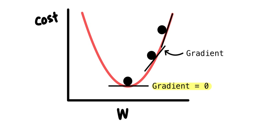
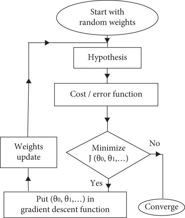
Gradient Descent:

Imagine you’re on a hill, blindfolded, and you want to get to the bottom (lowest loss). You touch the ground and feel which way is downhill — and take a tiny step. Do this again and again — that’s gradient descent.

Linear Regression isn’t just about drawing a line — it’s about learning the best one. That’s where Gradient Descent comes in.

Gradient Descent is an optimization technique. It starts with random values for β₀ and β₁ and slowly updates them to minimize the error (MSE).

The Update Rule:

Too big of a step, and you might miss the minimum. Too small, and learning takes forever. It’s a delicate balance.

Gradient Formula:

β₁ = β₁ - α × dJ/dβ₁
β₀ = β₀ - α × dJ/dβ₀

Where:

• α is how big your step is (learning rate)
• dJ/dβ is how steep the hill is at your spot (gradient)
• We subtract because we want to go downhill

Evaluating the Model:

After your robot is trained, how do you know if it’s actually good? We use two main tools:

MSE Lower MSE means your guesses are closer to the truth.

R² Score This tells you how much your model explains the data. R² = 1 means perfect fit R² = 0 means useless model

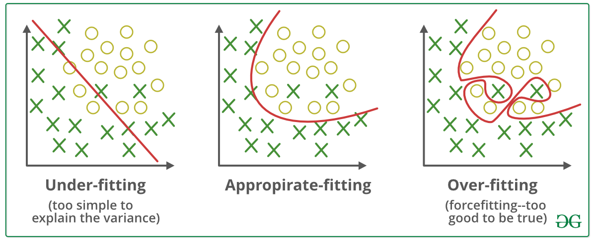
Overfitting vs Underfitting

Let’s say you’re drawing a line through points.

Just Right A smooth line that goes through the middle, this is just right.

Overfitting You try so hard to be perfect, you make a crazy zigzag line that fits every point, even noise or mistakes. Too smart = bad generalization. Example: Your model remembers training data like answers to a quiz, but fails new questions.

Underfitting You draw a straight line even when the data is clearly curved — your model is too simple. Example: Predicting house prices using only the number of windows, ignoring location, size, etc.

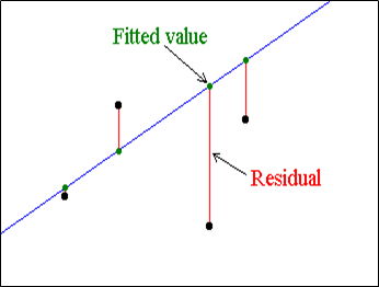
Residuals: What’s Left Behind?

A residual is the difference between the actual observed value and the value predicted by the model. Mathematically, it is: Residual = Actual - Predicted

If your model is good, the residuals should look random (like scattered dots above and below 0). If you see a curve in your residual plot — your model probably missed something.

residuals = y - y_pred
sns.residplot(x=y_pred, y=residuals, lowess=True)

Regularization (Preventing Overfitting)

When models become too fancy (with big numbers), they can overfit.

Regularization is like telling the model: “Hey! Don’t go too crazy with big numbers!”

Ridge Regression (L2) Adds penalty to large squared weights: + α × Σ(β²)

Lasso Regression (L1) Adds penalty to absolute weights: + α × Σ|β|

Polynomial Features (Fitting Curves)

Linear Regression fits straight lines. What if your data is curved? Use Polynomial Regression:

from sklearn.preprocessing import PolynomialFeatures
poly = PolynomialFeatures(degree=2)
X_poly = poly.fit_transform(X)

Now your input becomes [1, x, x²] — and your model can make curves.

Feature Scaling

If one feature is in meters and another is in grams, your model gets confused.

Scaling puts everything on the same scale.

from sklearn.preprocessing import StandardScaler
scaler = StandardScaler()
X_scaled = scaler.fit_transform(X)

This helps Gradient Descent work better and faster.

---

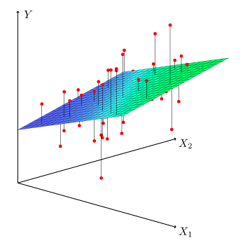
Multiple Linear Regression

Multiple Linear Regression is a statistical technique used to model the relationship between one dependent variable and two or more independent variables. It extends simple linear regression, which uses only one independent variable, by allowing for multiple predictors.

Multiple linear regression estimates the linear relationship between the dependent variable $y$ and multiple independent variables $x_1, x_2, \ldots, x_n$ using the following equation:

y = β₀ + β₁x₁ + β₂x₂ + … + βₙxₙ + ε

Where:

• y: Dependent variable (the value we want to predict)
• x_1, x_2, …, x_n: Independent variables (the predictors)
• β₀: Intercept term
• β₁, β₂, …, βₙ: Coefficients representing the impact of each independent variable
• ε: Error term (accounts for variability not explained by the model)

---

Purpose:

The goal of multiple linear regression is to find the best-fitting line (or hyperplane in higher dimensions) through the data points by minimizing the difference between the predicted values and the actual values of the dependent variable.

Example:

Suppose you want to predict a student’s final exam score based on the number of hours studied, number of hours slept, and attendance rate. The model might look like this:

Score = β0 + β1 × StudyHours + β2 × SleepHours + β3 × Attendance + ε

This model allows you to quantify how each factor contributes to the predicted score.

---

Now the most important question comes into our mind, when are we supposed to use this model? Out of so many models, how are we going to figure out when and where Linear Regression will fit in the best way?

To understand this, there are a few things we would have to consider first:

When to Use Linear Regression

Linear Regression works best under these conditions:

1. You want to predict a continuous numeric value

• Example: Predicting house price, temperature, or sales revenue.
• Not suitable for classification (e.g., spam vs. not spam).

2. There’s a linear relationship between variables

• The relationship between features (X) and target (y) should be roughly linear.
• Example: As square footage increases, price also increases steadily.

You can check this with:

3. The data meets these assumptions:

Assumptions of Linear Regression

https://www.geeksforgeeks.org/assumptions-of-linear-regression/

Before using linear regression, we make some assumptions:

1. Linearity: Relationship between the features and the target is linear.
2. Independence: Observations are independent of each other.
3. Homoscedasticity: Constant variance of residuals(The spread of errors).
4. Normality: The differences between the real and predicted values (residuals) should follow a normal distribution.
5. No multicollinearity: Features shouldn’t be too correlated with each other.

---

When Not to Use Linear Regression

Avoid Linear Regression in these situations:

1. The relationship is non-linear

• If the plot of X vs. y is curved, linear regression will underfit.
• Consider Polynomial Regression, Decision Trees, or Neural Networks.

2. There are major outliers

• Linear Regression is very sensitive to outliers.
• Use Robust Regression or clean your data beforehand.

3. Your features are highly correlated

• Multicollinearity makes it hard to understand feature importance.
• Use PCA, or Ridge/Lasso to regularize.

4. You’re solving a classification problem

• Linear regression is not meant for binary or multi-class classification.
• Use Logistic Regression, Random Forest, or SVM.

5. You need interpretability and your data breaks assumptions

• Linear Regression is interpretable but only when its assumptions hold.
• If assumptions break, you might draw wrong conclusions.

Closing Thoughts

Linear Regression may be called “simple,” but it teaches the foundations of machine learning. From assumptions to tuning, from math to code, it all starts here.

Mastering it opens doors to deeper understanding.

---